Home > 2. Marine GIS > 2.16 Grid Stats
2.16 Using Grid Statistics and Calculations for Ecological Assessments in Saga
|
|
|
1. Use the methods in Importing Unprojected HDF Satellite Imagery (L3/L4) into Marine GIS to download all 12 months of the Level 3 Sea Surface Temperatur (SST) climatologies (preferably 4-km resolution). Convert to TXT then ASC and then import them into Saga, as shown in the exercise.
NOTE: If you are really pressed for time, you can use only the January, April, July and October images. |
|
| 2. Use the methods in Resampling Grid Data to the Project Map Extent with a "Dummy" Grid to cut all 12 monthly grids down to the dimensions of the Liberia area of interest, using the 0.05-degree target grid. You can read the justification for this choice in the "grid scale" section of OceanTeacher article on gridded data (cited above). This grid is mandatory to keep the original resolution. Because they are so close (4 km versus 0.05 degrees) the resampling method can be NEAREST NEIGHBOR. | |
| 3. Use the methods in Converting Data Grids from Scaled Integers to Real Values to convert the Liberia area grids to actual temperature values. These are the only grids you really need to save, in the folder PRODUCTS > SAGA > GRIDS, with filenames like sst_apr_liberia_modisa_ocweb_11u_daytime_.05deg_hdfview_saga | |
| 4. You probably need to do a little housekeeping, and remove all data objects in Saga except the 12 final grids you just made. For now, save the huge BZ2, HDF, TXT and ASC files on your hard drive, until we're sure they were properly made and the analyses below will succeed. | |
| 5. All 12 monthly grids must be loaded into Saga. Proof of their identical structure (a requirement of this method) is demonstrated by their placement under one grid system. |  |
|
6. Select MODULES > GEOSTATISTICS-GRIDS > STATISTICS FOR GRIDS.
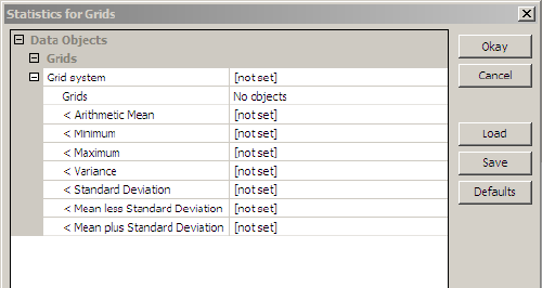
This module allows you to calculate any or all of the 7 statistical measures shown here, for example the ARITHMETIC MEAN. These measures, when they are SET, are calculated from all 12 monthly values of each pixel, and a new grid is created consisting of these statistical pixels. |
 |
|
7. For GRID SYSTEM select the system of the monthly SST grids.
Then click on the ellipsis (...) to the right of NO OBJECTS. |
 |
| 8. This grid object selection window appears. | 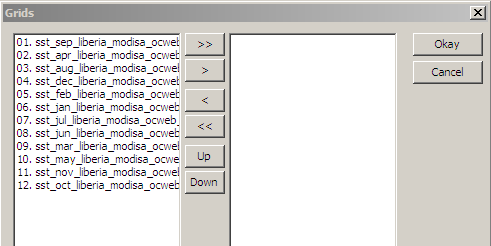 |
|
9. Click on the >> control to select all 12 grids. They will move to the right side, as you see here.
Then click OK. |
 |
| 10. Now you can select which statistics to create. Change the settings by ARITHMETIC MEAN, MINIMUM and MAXIMUM to CREATE. Then click OK. | 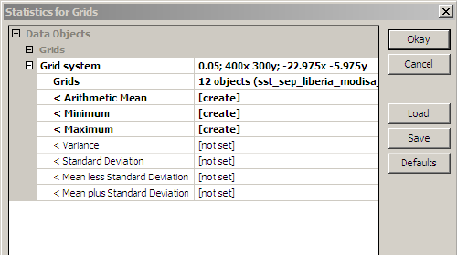 |
| 11. These new grids appear in the Saga data list. |  |
12. To preserve your work, you can use SAVE AS and save them in the folder PRODUCTS > SAGA > GRIDS with these names (where AVG denotes the ARITHMETIC MEAN)
|
|
13. You might also save the entire project at this stage, with FILE > PROJECT > SAVE PROJECT AS, and use the folder PRODUCTS > SAGA > PROJECTS, with this project name:
|
|
| 14. Here, for example, is the average value grid. It is probably exactly the same as the annual average HDF grid that you could have downloaded from the Ocean Color Web. |  |
|
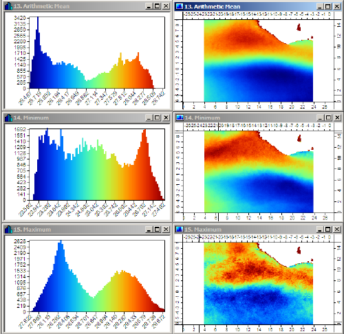
15. Here you can see all three statistical grids, with their histograms. In Saga the WINDOW > TILE VERTICALLY control sets up a display like this (but sometimes you must move an image or two).
This set of images looks interesting, but you must remember that the color scales are all automatically set by Saga, and may not "make sense" scientifically. |
 |
|
16. Here, the VALUE RANGE has been set to the same range for all figures. The lowest value is the lowest temperature in the MINIMUM grid (20 degrees). The highest value is the highest value in the MAXIMUM grid (30 degrees).
Now the figures can confidently be compared visually, and they "make sense" scientifically. You can simply check the single, unified color palette on the top right to estimate SST values for any figure. As a biologist, you could now use these grids to assess the highest and lowest temperatures that usually occur here, and where they occur. This is a very basic ecological concept that is much easier to do with these statistical images, than by visually scanning 12 (or more!) monthly images. |
 |
| 17. These figures are not the final end of this exercise. Now we're going to use them to derive some other products of ecological significance. | |
| 18. Select MODULES > GRID-CALCULUS > GRID CALCULATOR. |  |
|
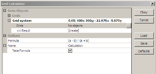
19. Once again, for GRID SYSTEM, select the same system as the monthly climatology grids.
Then click on the ellipsis (...) to the right of NO OBJECTS. |
 |
|
20. Select the MINIMUM and MAXIMUM grids with the > control. Notice that MINIMUM is first, so it is "grid a" in the Saga logic, and MAXIMUM is second, so it it "grid b".
Then click OK. |
 |
|
21. Now, in the calculator window, enter the FORMULA to apply, which is b-a. This means MAXIMUM minus MINIMUM.
You can set NAME to be ANNUAL RANGE, so the new grid has a clear identity. Then click OK. |
 |
| 22. The new grid ANNUAL IDENTITY will appear in the Saga data list. Before you look at it, go to the OPTIONS panel, and select COLORS. | |
|
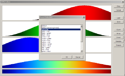
23. In the color selection window, select PRESET from the right-hand menu, then choose the GRAYSCALE from the available choices.
Then click OK and click OK. Then click SETTINGS > APPLY in the bottom of the OPTIONS panel. |
 |
|
24. Now, when you select and view the annual temperature range grid, it is not shown in a color palette. This insures that you do not confuse it, a mathematical result, with the actual temperature values above.
You can see that the southeast area experience the greatest changes during the year, while the area directly west of Liberia shows the smallest changes. |
 |
|
25. The above figure is quite good enough for scientific analyses, but we want to take this analysis one step further. What if you were asked to "map" the area where annual temperature changes are 4 degrees or more, for example. By "map" we mean to create a map that unambiguously shows exactly where that area is, and the user is not required to make guesses based on color shades.
How do you do that? |
|
| 26. One way to do it is by "classifying" the data. Select MODULES > GRID-TOOLS > CHANGE GRID VALUES. |  |
27 Make these selection:
Then click on the ellipsis (...) to the right of LOOKUP TABLE. |
 |
| 28. The initial table has these 3 columns, but only 2 rows. You can use a right-click on any table row to ADD NEW ROWS. | 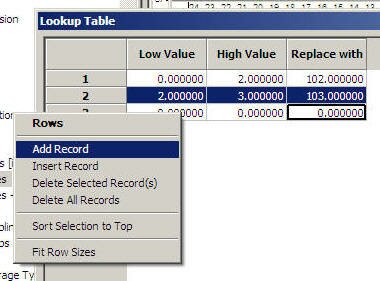 |
|
29. Edit the table to have these values:
Then click OK. And click OK again. |
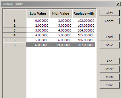 |
| 30. You now have a new grid named CHANGED GRID that does not contain SST values or SST difference values at all. It contains only numerical codes. Each pixel has been assigned a code to show where it is found in the above table. | |
| 30. Here is the histogram for CHANGED GRID, showing that it only has 4 different values. Apparently there were no values in the lowest or highest bins.. |  |
| 32. And here is the changed grid, a "classified grid", showing the different code zones. |  |
| 33. You might want to save this grid now, in the folder PRODUCTS > SAGA > GRIDS with the filename sst_classed_max_minus_min_annu_liberia_modisa_ocweb_11u_daytime_.05deg_hdfview_saga | |
|
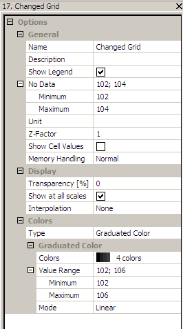
34. If you want to visualize only a portion of these zones, you can manipulate the NO DATA fields of the OPTIONS panel. This is possible, because the temperature range codes are sequential (an important thing to remember, if you do this sort of work).
Here the codes 102, 103 and 104 (covering temperature ranges from 0.0 to 4.0 degrees) are "masked" by declaring them to be NO DATA values. Click SETTINGS > APPLY to see the result. |
 |
|
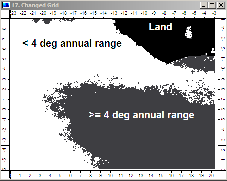
35. This is a map of the areas where the annual temperature range exceeds 4.0 degrees. [The land area of Liberia is also shown, because it has a value of -99999, the native NO DATA value in Saga.]
Maps like this are much more useful for decision-making and presentation, if you want to emphasize a particular area, rather than dazzle the viewer with colors. A standard graphics editor (IrfanView) has been used to add informative labels. |
 |
| 36. We hope you saw many possibilities in the above exercise for other statistical analyses that you can do with Saga. Once you have the library of basic grids (which is usually 95 % of the work), then the above steps are easy and fast. Good luck. | |